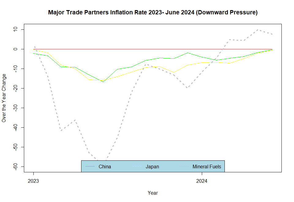
International trade contributes mixed signals on import prices as fuel and major trade partners’ prices offset each other. Prices for all import items from Canada, Mexico, and Europe increased by 3.2 percent on a yearly basis, while prices for all items from China and Japan remained negative at -0.5 percent over the year. Despite being negative figures, import prices for the latter two countries are on an upward trend. These data trends shed light on what monetary policy makers expect to see to make their minds before the following Federal Open Market Committee meeting on July 30th. Concerns over international supply chain lurk one more time.

Although import fuel prices decreased from May to June 2024, the series still contributes upward with change nearing eight percent over the year. The US Bureau of Labor Statistics reported on July 16th, 2024 that June Import prices were unchanged due mostly by the offsetting effect of fuel prices on monthly basis. However, a further major trade partner breakdown of the data provides a concerning signal of where prices are headed internationally and how inflation in the US may be affected.

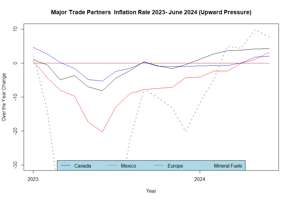
Mexico and Canada import prices have joined Europe’s upward trend since April, when reported data started showing positive changes not seen since the beginning of 2023. Not only have Canada and Mexico put pressure on US inflation lately, but also China and Japan have done so and are catching up rapidly on the trend, with a 0.17 and 0.04 monthly percent increase, respectively. These three months of consecutive increases may send a signal to support continued restrictive monetary policy measures (or at least unchanged) on the Federal Reserve side. Recent data on domestic prices show not only shelter, but also Communications and Food and Beverages are on the rise.

Assessing the chances for changes in current Monetary Policy seems feasible, although somewhat risky. At this point in time and overall, the Federal Reserve is looking at data on both the Job Market side and domestic prices that might support a reduction of Federal Funds rates, while the trade outlook looks slightly riskier than at the beginning of 2024.

_______________________

Code that generates the time series:

###################################################
###                                            ####
### Import and Export Prices BLS               ####
###                                            ####
###################################################




China_Manufacturing        <- blsR::get_series_table("EIUCDCHNMANU", start_year = 2020, end_year = 2024)
China_All                  <- blsR::get_series_table("EIUCDCHNTOT", start_year = 2020, end_year = 2024)
Canada_Manufacturing       <- blsR::get_series_table("EIUCDCANMANU",start_year = 2020, end_year = 2024)
Canada_All                 <- blsR::get_series_table("EIUCDCANTOT", start_year = 2020, end_year = 2024)
Europe_Union_Manufacturing <- blsR::get_series_table("EIUCDEECMANU", start_year = 2020, end_year = 2024)
Europe_All                 <- blsR::get_series_table("EIUCDEECTOT", start_year = 2020, end_year = 2024)
Japan_Manufacturing        <- blsR::get_series_table("EIUCDJPNMANU", start_year = 2020, end_year = 2024)
Japan_All                  <- blsR::get_series_table("EIUCDJPNTOT", start_year = 2020, end_year = 2024)
Mexico_Manufacturing       <- blsR::get_series_table("EIUCDMEXMANU", start_year = 2020, end_year = 2024)
Mexico_All                 <- blsR::get_series_table("EIUCDMEXTOT",  start_year = 2020, end_year = 2024)
Petroleum_Refineries       <- blsR::get_series_table("EIUIP2709",  start_year = 2020, end_year = 2024)
Mineral_Fuels              <- blsR::get_series_table("EIUIP27",  start_year = 2020, end_year = 2024)



Date_Parser <- function(Data){
  Real_Estate_Comp <- Data
  Real_Estate_Comp$Date <- as.Date(paste("01", Real_Estate_Comp$periodName, Real_Estate_Comp$year), tryFormats = "%d %B %Y")
  Real_Estate_Comp
}


Inflation_Calculator <- function(Data){
  Price_Index <- Data
  
  Price_Index$Laged_Year_Value      <- Price_Index[as.numeric(rownames(Price_Index))+12,]$value
  Price_Index$Over_Year_Inflation   <- ((Price_Index$value - Price_Index$Laged_Year_Value)/Price_Index$value)*100
  
  Price_Index$Laged_Month_Value     <- Price_Index[as.numeric(rownames(Price_Index))+1,]$value
  Price_Index$Over_Month_Inflation  <- ((Price_Index$value - Price_Index$Laged_Month_Value)/Price_Index$value)*100
  Price_Index
}


China_Manufacturing <- Date_Parser(China_Manufacturing)
China_Manufacturing <- Inflation_Calculator(China_Manufacturing_2)

China_All           <- Date_Parser(China_All)
China_All           <- Inflation_Calculator(China_All)


Canada_Manufacturing           <- Date_Parser(Canada_Manufacturing)
Canada_Manufacturing           <- Inflation_Calculator(Canada_Manufacturing)

Canada_All           <- Date_Parser(Canada_All)
Canada_All           <- Inflation_Calculator(Canada_All)

Japan_Manufacturing <- Date_Parser(Japan_Manufacturing)
Japan_Manufacturing <- Inflation_Calculator(Japan_Manufacturing)

Japan_All           <- Date_Parser(Japan_All)
Japan_All           <- Inflation_Calculator(Japan_All)

Mexico_Manufacturing <- Date_Parser(Mexico_Manufacturing)
Mexico_Manufacturing <- Inflation_Calculator(Mexico_Manufacturing)

Mexico_All           <- Date_Parser(Mexico_All)
Mexico_All           <- Inflation_Calculator(Mexico_All)

Europe_All           <- Date_Parser(Europe_All)
Europe_All           <- Inflation_Calculator(Europe_All)

Petroleum_Refineries <- Date_Parser(Petroleum_Refineries)
Petroleum_Refineries <- Inflation_Calculator(Petroleum_Refineries)



Mineral_Fuels       <- Date_Parser(Mineral_Fuels)
Mineral_Fuels       <- Inflation_Calculator(Mineral_Fuels)

Mineral_Fuels$Benchmark <- 0

plot(Mineral_Fuels$Over_Month_Inflation ~ Mineral_Fuels$Date, type= "l")

plot(Mineral_Fuels$Benchmark[1:18]~ Mineral_Fuels$Date[1:18], type = "l",
     ylim=c(-30,10), 
     col="brown",
     xlab = "Year",
     ylab = "Over the Year Change",
     main= "Major Trade Partners  Inflation Rate 2023- June 2024 (Upward Pressure)")
#lines(China_All$Over_Year_Inflation[1:18] ~ China_All$Date[1:18], col= "green")
lines(Canada_All$Over_Year_Inflation[1:18] ~ Canada_All$Date[1:18], col= "blue")
lines(Mexico_All$Over_Year_Inflation[1:18] ~ Mexico_All$Date[1:18], col= "red")
lines(Europe_All$Over_Year_Inflation[1:18] ~ Europe_All$Date[1:18], col= "black")
#lines(Japan_All$Over_Year_Inflation[1:18] ~ Japan_All$Date[1:18], col= "yellow")
lines(Mineral_Fuels$Over_Year_Inflation[1:18]~ Mineral_Fuels$Date[1:18], col= "grey",lty=3, lwd=3)
#lines(Mineral_Fuels$Benchmark[1:18]~ Mineral_Fuels$Date[1:18], type = "l", col="brown")
legend("bottom",c("Canada", "Mexico", "Europe", "Mineral Fuels"), 
       col= c("blue", "red", "black", "grey"),
       #pch=c("o","*","+"),
       lty=c(1,2,3,4),
       ncol = 4,
       bg="lightblue")


plot(Mineral_Fuels$Benchmark[1:18]~ Mineral_Fuels$Date[1:18], type = "l",
     ylim=c(-60,10), 
     col="brown",
     xlab = "Year",
     ylab = "Over the Year Change",
     main= "Major Trade Partners Inflation Rate 2023- June 2024 (Downward Pressure)")
lines(China_All$Over_Year_Inflation[1:18] ~ China_All$Date[1:18], col= "green")
#lines(Canada_All$Over_Year_Inflation[1:18] ~ Canada_All$Date[1:18], col= "blue")
#lines(Mexico_All$Over_Year_Inflation[1:18] ~ Mexico_All$Date[1:18], col= "red")
#lines(Europe_All$Over_Year_Inflation[1:18] ~ Europe_All$Date[1:18], col= "black")
lines(Japan_All$Over_Year_Inflation[1:18] ~ Japan_All$Date[1:18], col= "yellow")
lines(Mineral_Fuels$Over_Year_Inflation[1:18]~ Mineral_Fuels$Date[1:18], col= "grey",lty=3, lwd=3)
#lines(Mineral_Fuels$Benchmark[1:18]~ Mineral_Fuels$Date[1:18], type = "l", col="brown")
legend("bottom",c("China", "Japan", "Mineral Fuels"), 
       col= c("green", "yellow", "grey"),
       #pch=c("o","*","+"),
       lty=c(1,2,3),
       ncol = 3,
       bg="lightblue")

mean(c(Canada_All$Over_Year_Inflation[1], Mexico_All$Over_Year_Inflation[1], Europe_All$Over_Year_Inflation[1]))
mean(c(China_All$Over_Year_Inflation[1], Japan_All$Over_Year_Inflation[1]))


China_All$Sequence <- seq(1:54)
Japan_All$Sequence <- seq(1:54)

lm(China_All$Over_Month_Inflation[1:5] ~ China_All$Sequence[1:5])
lm(Japan_All$Over_Month_Inflation[1:5] ~ Japan_All$Sequence[1:5])

Automated Data Reports? Make an Appointment