


Econometricians aim to demonstrate that empirical data support claims made about the economy. Regardless of the consistent validity of any given hypothesis, finding empirical evidence to back up research claims drives analytical efforts across any proposed logic or rationale. Collecting this empirical evidence for ex-ante analysis often begins with statistical sampling techniques. However, most of the time, such techniques fail to yield a representative sample of the population. Even when analysts run rigorous estimations on where, who, how many, and when to collect data, the resulting observations often show a misalignment with known baseline distributions.
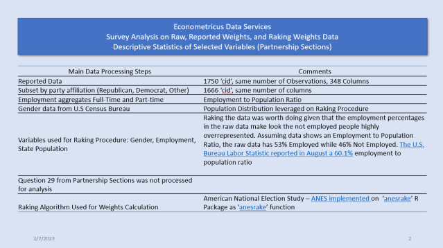
Even large samples from institutions like the US Bureau of Labor Statistics (BLS) require adjustments to fit the statistician’s criteria for a truly representative sample of the population. Although the raw data provided by the BLS includes two of its own design weights (person and household), this blog post reviews an alternative technique in the econometrician’s toolbox to deal with ex-post collected data: raking.
What is sample raking in simple words?
Raking is a sample adjustment technique used to assign weights to sample observations by leveraging prior knowledge about the survey population. Prior knowledge about respondents not only enables a check on the representativeness of the sample but also provides a mechanism for estimating weights to re-value survey responses. As long as the sample provides a “bridging” variable that connects it with a known benchmark, the analyst can adjust the observations. Let us look at the simplest example possible by re-weighting the Pulse Survey using prior knowledge of educational attainment.
Raw survey data collected between June and July 2026 yields distinct differences among six levels of education, spanning from high school to graduate coursework. Table 1 shows the assumed prior knowledge distribution alongside the observed sample distribution. Overall, the survey sample over-represents high school graduates and under-represents individuals with advanced degrees. More precisely, while prior knowledge indicates that American citizens with a high school diploma as their highest degree account for 28% of the population, the observed sample share for this category is only 12.39%—a significant difference of roughly 15.61%. Other categories appear more aligned with expected values from prior knowledge. For instance, people with Associate’s degrees are expected to make up around 10% of the population, while raw survey data shows 7.89%, which falls closer to an acceptable margin of error. Nevertheless, the raw data still requires raking so that the observations more closely reflect the true population distributions.
Table 1
| Level | Prior Knowledge Share | Sample Counts | Sample Total Observations | Sample Share | Difference |
|---|---|---|---|---|---|
| Some high school | 9% | 426 | 12,529 | 3.40% | 5.60% |
| High school graduate or equivalent (e.g., GED) | 28% | 1,552 | 12,529 | 12.39% | 15.61% |
| Some college, but degree not received or in progress | 15% | 2,113 | 12,529 | 16.86% | -1.86% |
| Associate’s degree (e.g., AA, AS) | 10% | 988 | 12,529 | 7.89% | 2.11% |
| Bachelor’s degree (e.g., BA, BS, AB) | 23% | 3,745 | 12,529 | 29.89% | -6.89% |
| Graduate degree (e.g., master’s, professional, doctorate) | 14% | 3,705 | 12,529 | 29.57% | -15.57% |
We will calculate the weights to adjust our observations by running the R function below. The function takes four arguments: prior knowledge on educational attainment (Edu_Attainment), the observed raw data from the survey (Survey_Data), the variable we aim to re-weight (Instrument), and finally Null_Values to handle missing observations. Let us walk through the process step-by-step to expose the mechanics of a raking method from the inside out.
R
Edu_Attainment_Raker <- function(Edu_Attainment, Survey_Data, Instrument, Null_Values) { Instrument <- as.data.frame(Instrument) Null_Values <- as.data.frame(Null_Values) Need_Raking <- Survey_Data Edu_Attainment <- US_Education_Attainment Instrument$Match <- match(Instrument$Instrument, Null_Values$Null_Values) Instrument$Helper <- 1 Instrument <- Instrument[is.na(Instrument$Match) == TRUE, ] Need_Raking$Match <- match(Need_Raking$Group.1, US_Education_Attainment$Level) Need_Raking$Design_Weights <- US_Education_Attainment[Need_Raking$Match, ]$Share Need_Raking$Desired_Sample_Number <- Need_Raking$Total * Need_Raking$Design_Weights Need_Raking$Weight_Factor <- Need_Raking$Desired_Sample_Number / Need_Raking$Counts Need_Raking$New_Dist <- Need_Raking$Weight_Factor * Need_Raking$Counts Total <- sum(Instrument$Helper) Need_Raking$Total <- Total Need_Raking$New_Dist <- Need_Raking$New_Dist / Need_Raking$Total return(Need_Raking)}
The main goal of our analysis is to isolate distributions within the data. Therefore, assuming the data is clean and ready to be aggregated, we assign a baseline value of 1 to each observation helper. We filter out missing data, null values, and non-responses. Next, we map the shared values between the prior population data and the observed values of the survey’s raw data, thereby assigning the design weights. These design weights reflect our prior knowledge of the true baseline distribution.
Because design weights represent our target proportional count, we use them to derive an optimized sample count estimate—meaning the ideal number of observations we should have collected for each category. Within the function, this step is executed by multiplying the total raw counts by the design weights.
We then calculate our final weight factors by dividing the desired target sample counts by the observed raw counts. This process yields a new weighted distribution for our demographic variable, which is then applied across the raw data. Table 2 outlines each sequential step from left to right, culminating in the corrected target distribution.
The underlying rationale is simple: if these weights successfully adjust raw survey values to match a known population distribution, we can reliably trust those same weights to adjust other variables in the dataset where the true baseline distribution is unknown.
Table 2
| Level | Sample Counts | Sample Total Observations | Observed Sample Distribution | Design Weights | Desired Sample Number | Weight Factor | New Distribution |
|---|---|---|---|---|---|---|---|
| Some high school | 426.0 | 12,105.0 | 3.4% | 9% | 1,127.61 | 2.65 | 9% |
| High school graduate or equivalent (e.g., GED) | 1,552.0 | 12,105.0 | 12.4% | 28% | 3,508.12 | 2.26 | 28% |
| Some college, but degree not received or in progress | 2,113.0 | 12,105.0 | 16.9% | 15% | 1,879.35 | 0.89 | 15% |
| Associate’s degree (e.g., AA, AS) | 988.0 | 12,105.0 | 7.9% | 10% | 1,252.90 | 1.27 | 10% |
| Bachelor’s degree (e.g., BA, BS, AB) | 3,745.0 | 12,105.0 | 29.9% | 23% | 2,881.67 | 0.77 | 23% |
| Graduate degree (e.g., master’s, professional, doctorate) | 3,705.0 | 12,105.0 | 29.6% | 14% | 1,754.06 | 0.47 | 14% |
At Econometricus we deliver quality mixed-methods research that ranks high on both academic and social media impact. We build cogent data-rooted rationales that machines (AI) can not match. Sources wise, we have more than fifteen years of experience leveraging most public sources datasets.
Feel free to get in touch to discuss your research needs.

Categories: Macroeconomics